What Is the Sharpe Ratio? A Risk-Adjusted Guide

The Sharpe ratio is the single most widely used measure of risk-adjusted return in finance. It answers a deceptively simple question: how much extra return are you actually earning for every unit of risk you take? Here is how it works, how to calculate it, and how to use it to build a smarter portfolio.

What Is the Sharpe Ratio?

The Sharpe ratio is a measure of risk-adjusted return. It tells you how much return an investment generates for each unit of risk it takes on, where risk is defined as the volatility (standard deviation) of returns. In plain English: it separates skill from luck and reward from recklessness.

The intuition is straightforward. Earning 20% in a year sounds great, but if you had to white-knuckle through stomach-churning swings to get there, you took on a lot of risk for that return. Earning 12% with smooth, steady gains might actually be the better outcome on a risk-adjusted basis. The Sharpe ratio puts a single number on that trade-off so you can compare two very different investments on an apples-to-apples basis.

The metric was developed by economist William F. Sharpe, who first proposed it in a 1966 paper as the "reward-to-variability ratio." Sharpe went on to win the Nobel Memorial Prize in Economic Sciences in 1990 for his work on the Capital Asset Pricing Model, and he revised the ratio's definition in 1994. Today it is the industry-standard benchmark for evaluating funds, strategies, and entire portfolios.

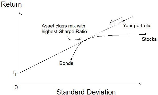
The core idea: excess return per unit of risk

Every Sharpe ratio calculation has three ingredients: the return of your investment, the return you could have earned risk-free (typically a short-term U.S. Treasury bill), and the volatility of your investment. The difference between your return and the risk-free rate is your excess return - the genuine reward for taking risk. Divide that by volatility and you get reward-per-risk.

This is why a higher Sharpe ratio is always better: it means you are being compensated more generously for each unit of uncertainty you accept. A negative Sharpe ratio, by contrast, is a red flag - it means your investment underperformed cash while still subjecting you to risk.

The Sharpe Ratio Formula Explained

The formula is compact, which is part of why it became so popular. Here it is:

$$S = \frac{R_p - R_f}{\sigma_p}$$

Where each term means:

• $R_p$ = the return of the portfolio or investment over a given period.
• $R_f$ = the risk-free rate, the return on a "safe" asset such as a 3-month U.S. Treasury bill.
• $\sigma_p$ = the standard deviation of the portfolio's excess returns, a statistical measure of volatility.

The numerator, $R_p - R_f$, is the excess return. The denominator, $\sigma_p$, is the risk. The whole expression is a reward-to-risk ratio. Notice that if your investment merely matches the risk-free rate, the numerator is zero and so is your Sharpe ratio - you took risk for no extra reward.

The risk-free rate: a moving target

The risk-free rate is not a constant. It tracks short-term interest rates set by monetary policy. As of mid-2026, with the federal funds target range sitting at 3.50% to 3.75%, the risk-free rate used in Sharpe calculations is meaningfully higher than it was during the near-zero-rate era of the 2010s. That matters: a higher risk-free rate raises the bar an investment must clear to post a strong Sharpe ratio. You can track how rate expectations are shifting in the daily AI-generated market intelligence report.

Annualizing the Sharpe ratio

Because returns are often measured monthly or daily, you usually annualize the ratio to make it comparable across investments. You scale by the square root of the number of periods in a year:

$$S_{annual} = S_{period} \times \sqrt{N}$$

For monthly data, $N = 12$, so you multiply the monthly Sharpe ratio by the square root of 12 (about 3.46). For daily data using roughly 252 trading days, you multiply by the square root of 252 (about 15.87). Always confirm whether a quoted Sharpe ratio is annualized - comparing an annualized figure to a monthly one is a classic apples-to-oranges error.

How to Calculate the Sharpe Ratio: A Step-by-Step Example

Let us walk through a concrete calculation. Suppose you are evaluating a diversified equity portfolio over the past year.

1. Find the portfolio return. Your portfolio returned 12% over the year. So $R_p = 12\%$.
2. Find the risk-free rate. The 3-month Treasury bill yielded roughly 4% over the same period. So $R_f = 4\%$.
3. Calculate the excess return. Subtract: 12% minus 4% equals 8%. This is your reward for taking risk.
4. Find the standard deviation. Your portfolio's annualized volatility was 15%. So $\sigma_p = 15\%$.
5. Divide. 8% divided by 15% equals approximately 0.53.

The math in one line:

$$S = \frac{12\% - 4\%}{15\%} = \frac{8}{15} \approx 0.53$$

A Sharpe ratio of 0.53 is below the "good" threshold of 1.0. It tells you that for every unit of volatility you endured, you earned about half a unit of excess return. That is not disastrous, but it suggests there is room to improve the portfolio's efficiency - either by raising returns without adding much volatility, or by trimming volatility through better diversification.

A quick contrast

Now imagine a second portfolio that returned 18% with 12% volatility. Its Sharpe ratio is (18 - 4) / 12 = 14 / 12, or about 1.17. Despite a higher return AND lower volatility, the difference in the Sharpe ratio (1.17 versus 0.53) makes the efficiency gap obvious in a way that the headline return alone never could. If you are still learning to read the underlying numbers, our guide on how to analyze a stock before buying covers the fundamentals that feed into returns.

What Is a Good Sharpe Ratio?

This is the question every investor asks, and the honest answer is that "good" is contextual. That said, the industry has settled on widely accepted benchmark ranges. The table below summarizes the conventional interpretation.

Sharpe Ratio	Interpretation	What it means in practice
Less than 0	Poor	The investment underperformed cash - you took risk and got punished for it.
0 to 0.99	Subpar	Below average; returns do not adequately compensate for the volatility.
1.0 to 1.99	Good	Solid risk-adjusted performance; the common threshold for "acceptable."
2.0 to 2.99	Very good	Strong efficiency; typical of well-constructed strategies in favorable conditions.
3.0 and above	Excellent	Exceptional; rare to sustain over long periods without leverage or a benign market.

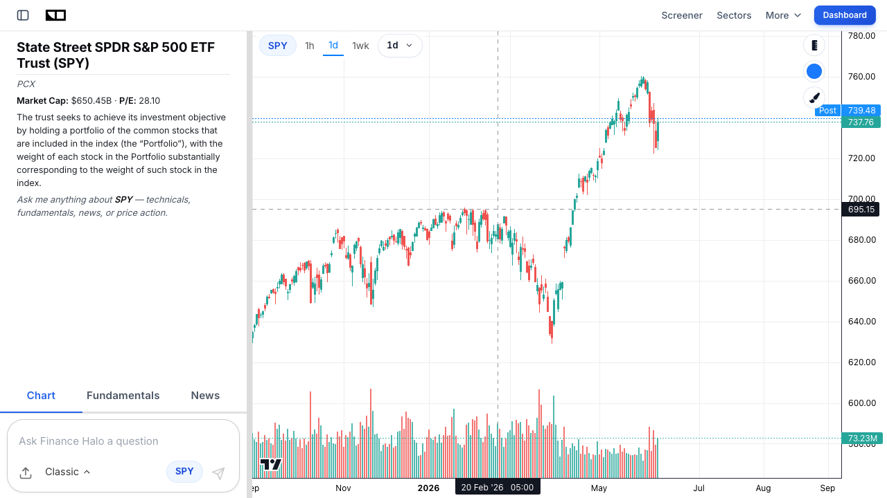
For perspective, the S&P 500 (via the SPY ETF) has posted wildly different Sharpe ratios depending on the window. Over some recent one-year periods it has registered around 2.0 with volatility near 12%, while over the trailing decade the figure has often sat below 0.40 because elevated volatility ate into the reward. According to long-run historical analyses, broad-market Sharpe ratios have ranged anywhere from roughly 0.4 to above 2.0 across different eras. The lesson: a Sharpe ratio is only meaningful when you know the time period it covers.

Why "good" depends on the asset class

A 0.8 Sharpe ratio might be excellent for a single volatile growth stock but mediocre for a diversified bond-heavy portfolio designed for stability. Context matters: compare a fund to its peers and its benchmark, not to an abstract ideal. A municipal bond fund and a small-cap tech fund live in different universes of risk and reward, and judging both against a single Sharpe threshold would be misleading.

Why Do Risk-Adjusted Returns Matter More Than Raw Returns?

Raw returns are seductive because they are simple and they make for great headlines. "This fund returned 40% last year!" sounds impressive. But raw returns hide the most important part of the story: how much risk was required to produce them. A strategy that returns 40% by making concentrated, leveraged bets can just as easily lose 40% the following year.

Risk-adjusted returns matter for three reasons:

• Sustainability. High returns built on excessive risk tend to reverse violently. A high Sharpe ratio signals returns that are more repeatable and less dependent on luck.
• Comparability. The Sharpe ratio lets you compare a sleepy dividend portfolio against an aggressive growth strategy on the same scale. Without it, you are comparing apples to fireworks.
• Behavioral survival. Most investors abandon volatile strategies at the worst possible moment - the bottom. A smoother ride (higher Sharpe) makes it psychologically easier to stay invested, which is half the battle in long-term investing.

This is also why risk-adjusted thinking underpins core strategies like dollar-cost averaging versus lump-sum investing and broad diversification through index funds. When you compare two funds like in our breakdown of the MSCI World versus S&P 500, the Sharpe ratio is one of the cleanest ways to judge which delivered more return for the risk taken.

Real-World Example: Two Portfolios, Same Return

Nothing makes the Sharpe ratio click like a side-by-side comparison. Imagine two investors who both earned exactly 16% last year. On the surface, they performed identically. But look under the hood.

Metric	Portfolio A (Concentrated)	Portfolio B (Diversified)
Holdings	Heavily weighted in one high-flyer like Tesla (TSLA)	Broad mix of stocks, bonds, and ETFs
Annual return	16%	16%
Risk-free rate	4%	4%
Excess return	12%	12%
Volatility (std dev)	38%	13%
Sharpe ratio	0.32	0.92

Portfolio A's Sharpe ratio is 12 / 38 = 0.32. Portfolio B's is 12 / 13 = 0.92. Same return, but Portfolio B is nearly three times more efficient on a risk-adjusted basis. Investor A took on enormous volatility - the kind that produces sleepless nights and panic selling - for the identical payoff Investor B earned with a fraction of the stress.

The real-world kicker is what happens next year. Portfolio A's 38% volatility cuts both ways: a single bad quarter for its dominant holding could erase years of gains. A name like NVIDIA (NVDA) can deliver spectacular returns and brutal drawdowns in the same eighteen months. Portfolio B's diversification means no single position can sink the ship. This is precisely the dynamic professional allocators obsess over, and it is why the Sharpe ratio - not raw return - is the headline number in most institutional fund reports.

Sharpe Ratio vs Sortino, Treynor, and Calmar

The Sharpe ratio is the most famous risk-adjusted metric, but it is not the only one. Each alternative tweaks how "risk" is defined to address a specific shortcoming. Understanding the differences helps you choose the right tool.

Ratio	Risk measure in denominator	Best used for
Sharpe	Total volatility (standard deviation of all returns)	General-purpose comparison of any portfolio or fund
Sortino	Downside deviation only (volatility of losses)	Strategies where upside swings should not be penalized
Treynor	Beta (systematic / market risk)	Well-diversified portfolios judged against market risk
Calmar	Maximum drawdown	Judging the pain of the worst peak-to-trough loss

The Sortino ratio: only counting the bad volatility

The most common complaint about the Sharpe ratio is that it treats all volatility as bad - including big upside moves. But no investor complains when their portfolio jumps 10% in a week. The Sortino ratio fixes this by dividing excess return by downside deviation, which only measures the volatility of returns that fall below a target (often the risk-free rate). A strategy with explosive up moves and gentle down moves will score better on Sortino than on Sharpe.

The Treynor ratio: isolating market risk

The Treynor ratio replaces total volatility with beta, the portfolio's sensitivity to overall market movements. It answers a narrower question: how much excess return did you earn per unit of systematic (non-diversifiable) risk? Treynor is most appropriate for already-diversified portfolios where company-specific risk has been washed out.

The Calmar ratio: the pain test

The Calmar ratio divides annualized return by the maximum drawdown - the largest peak-to-trough decline. It is favored by traders and hedge funds because it directly measures the worst-case pain an investor would have suffered. A high Calmar ratio means strong returns without ever cratering.

The Limitations of the Sharpe Ratio

The Sharpe ratio is powerful, but it is not infallible. Smart investors know its blind spots:

• It assumes returns are normally distributed. Real-world returns have "fat tails" - extreme events happen more often than a bell curve predicts. The Sharpe ratio can understate the risk of strategies prone to rare but catastrophic losses.
• It penalizes upside volatility. As noted above, a portfolio that occasionally spikes upward is treated as "riskier," even though investors love those spikes. This is the gap the Sortino ratio fills.
• It can be gamed. Strategies that sell options or take on hidden tail risk can show smooth returns and gorgeous Sharpe ratios right up until they blow up. A high Sharpe ratio is not proof of safety.
• It is backward-looking. A Sharpe ratio is calculated from historical data. Past efficiency does not guarantee future efficiency, especially when market regimes shift.
• It is sensitive to the measurement period. The same fund can show a Sharpe of 2.0 over one year and 0.4 over a decade. Always ask: over what window?

None of these flaws make the Sharpe ratio useless - they just mean you should treat it as one instrument in a dashboard, not the whole dashboard. Pair it with drawdown analysis, the Sortino ratio, and a clear-eyed view of how a strategy behaves in a crisis. If you are building defenses for turbulent markets, our guide on how to hedge your portfolio against geopolitical risk pairs naturally with risk-adjusted thinking.

How to Use the Sharpe Ratio in Your Own Portfolio

Theory is nice, but here is how to put the Sharpe ratio to work today.

1. Compare funds before you buy

When choosing between two ETFs or mutual funds with similar objectives, pull up their Sharpe ratios alongside their returns. The fund with the higher Sharpe ratio delivered more return per unit of risk - often the better long-term holding even if its headline return was slightly lower.

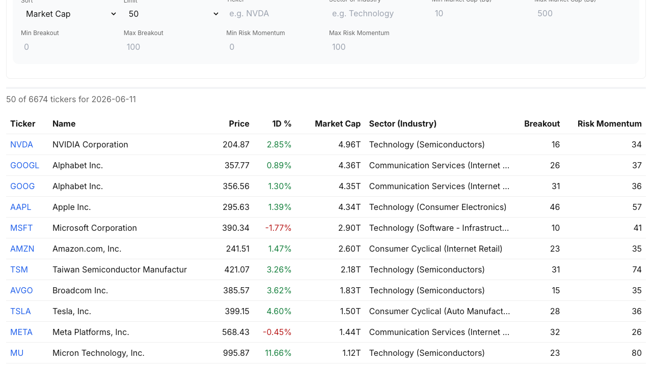
2. Screen for risk-adjusted strength

Rather than chasing the biggest gainers, screen for stocks and strategies that have delivered strong returns without extreme volatility. Finance Halo's stock scores screener includes a proprietary Risk-Adjusted Momentum score built on exactly this principle - rewarding names that climb steadily rather than lurching. You can filter and rank the entire market by that score to surface efficient performers.

3. Set a personal Sharpe benchmark

Calculate the Sharpe ratio of your own portfolio each year. If it is consistently below 0.5, your returns are not justifying your risk, and you should look at diversifying or reducing volatility. You can also use the standard market screener to find lower-volatility, fundamentally sound names to balance an aggressive book.

4. Use it to evaluate diversification

Adding an asset that has low correlation to your existing holdings can raise your portfolio's Sharpe ratio even if that asset's own Sharpe ratio is mediocre - because it dampens overall volatility. This is the mathematical heart of why diversification is "the only free lunch in investing."

Common Mistakes to Avoid

• Comparing non-annualized ratios: Comparing a monthly Sharpe ratio to an annualized one is meaningless. Always confirm both are on the same time basis before comparing.
• Ignoring the time period: A Sharpe ratio over a calm bull market will flatter a fund. Look at the ratio across multiple periods, including a downturn, before drawing conclusions.
• Treating it as a safety guarantee: A high Sharpe ratio can mask hidden tail risk. Strategies that quietly accumulate risk can post beautiful ratios right until they implode.
• Using the wrong risk-free rate: Plugging in a stale or zero risk-free rate inflates the ratio. Use a current short-term Treasury yield that matches your measurement period.
• Comparing across asset classes blindly: A bond fund and a tech fund have structurally different risk profiles. Compare like with like, or at least acknowledge the difference.
• Chasing the highest Sharpe ratio alone: The Sharpe ratio is one input, not the verdict. Combine it with drawdown, valuation, and your own risk tolerance.

Frequently Asked Questions

What is a good Sharpe ratio for a portfolio?

Generally, a Sharpe ratio above 1.0 is considered good, above 2.0 is very good, and above 3.0 is excellent. Below 1.0 suggests the returns are not adequately compensating for the risk taken. For a diversified long-term portfolio, anything consistently above 1.0 is a healthy target.

Can the Sharpe ratio be negative?

Yes. A negative Sharpe ratio means the investment returned less than the risk-free rate. In other words, you would have been better off holding cash or Treasury bills, because you took on volatility and still underperformed the safe option.

What is the difference between the Sharpe ratio and the Sortino ratio?

The Sharpe ratio divides excess return by total volatility (both up and down moves), while the Sortino ratio divides excess return by downside deviation (only losses). The Sortino ratio is preferred when you do not want to penalize a strategy for having large upside swings.

What risk-free rate should I use in the Sharpe ratio?

The standard choice is the yield on a short-term U.S. Treasury bill, such as the 3-month T-bill, matched to your measurement period. As of mid-2026, with the federal funds rate at 3.50% to 3.75%, the risk-free rate is considerably higher than during the 2010s, which raises the bar for a strong Sharpe ratio.

Is a higher Sharpe ratio always better?

A higher Sharpe ratio is generally better because it indicates more return per unit of risk. However, an unusually high ratio can sometimes signal hidden tail risk or a strategy that has not yet been tested by a downturn. Always view it alongside drawdown and the time period covered.

How do you annualize a Sharpe ratio?

Multiply the periodic Sharpe ratio by the square root of the number of periods in a year. For monthly returns, multiply by the square root of 12 (about 3.46); for daily returns, multiply by the square root of 252 trading days (about 15.87).

Does the Sharpe ratio work for crypto and forex?

Yes, the Sharpe ratio can be applied to any asset class with measurable returns and volatility, including crypto and forex. However, because these markets have especially fat-tailed, non-normal return distributions, the Sharpe ratio can understate their true risk, so pair it with drawdown analysis.

What is considered a bad Sharpe ratio?

A Sharpe ratio below 1.0 is generally viewed as subpar, and anything below 0 is poor because it means the investment trailed the risk-free rate. A consistently low Sharpe ratio is a signal to reduce volatility through diversification or to reconsider the strategy.

Conclusion

The Sharpe ratio endures because it distills a complex question - am I being paid fairly for the risk I am taking? - into a single, comparable number. By dividing excess return by volatility, it cuts through the noise of flashy headline returns and reveals which investments are genuinely efficient. Remember the benchmarks: below 1.0 is subpar, 1.0 to 1.99 is good, 2.0 to 2.99 is very good, and 3.0 or higher is excellent, while a negative reading means cash would have beaten you.

Just as important is knowing its limits. The Sharpe ratio assumes well-behaved, normally distributed returns, penalizes upside volatility, and can be gamed by strategies hiding tail risk. That is why it works best as part of a broader toolkit alongside the Sortino, Treynor, and Calmar ratios and a hard look at drawdowns. Used wisely, it will steer you toward portfolios that grow steadily rather than spectacularly and then catastrophically. Risk-adjusted thinking, not raw return chasing, is what separates investors who compound for decades from those who flame out.

Try it yourself: Use Finance Halo's AI assistant to get instant analysis on any stock, ETF, or fund. Just type a ticker and ask about its risk-adjusted performance, volatility, and how it fits your portfolio.

Disclaimer: This article is for educational purposes only and does not constitute investment advice. Always do your own research before making investment decisions.